Clustering - Customer Personality (K-means/PCA)

Wondering how to segment your customers using raw data? In this article, I’ll show you how to create customer clusters based on personality profiles and tailor your marketing strategies for each segment. Let’s dive into data-driven insights!

We perform a Customer Personality Analysis to gain insights into the customer base of a company, using data provided from a kaggle dataset. You can find, download and modify all my code on my Kaggle :

Clustering : Customer Personality (K-means/PCA)

The primary objective of this analysis is to identify customer segments based on their purchasing habits and demographics. This segmentation will allow for more targeted marketing campaigns and better product recommendations. Using techniques like exploratory data analysis (EDA) and clustering algorithms, we will uncover key patterns and divide the customer base into distinct groups that exhibit similar behaviors.

Exploratory Data Analysis

Before diving into clustering, it’s essential to understand the structure of the data. The EDA provides a clear picture of the customer base's demographics, income distribution, and spending patterns.

Age Distribution

The dataset contains customers with a wide age range. To better visualize this, I plotted a histogram of the age distribution.

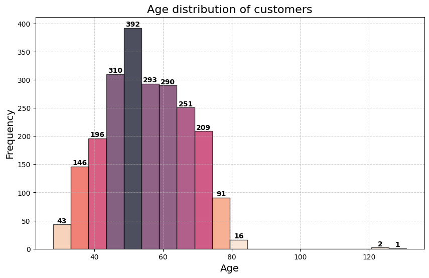
Insight: The age distribution shows that most customers are aged between 40 and 65, with very few customers older than 80.

Income Distribution (After Removing Outliers)

To visualize the income distribution, we plotted the customers whose income is below 100,000.

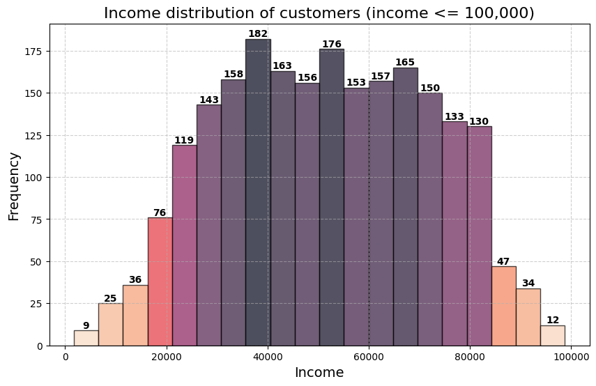
Insight: A very small percentage of customers (0.54%) have an income exceeding 100,000, which are treated as outliers.

Next, I removed outliers for income values above 300,000 and age values above 90, which helped focus the analysis on more realistic customer profiles.

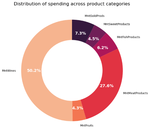
Spending Patterns on Products

We will analyze how much customers spend across various product categories

Preprocessing Data

Feature Engineering

Several features were engineered to enhance our model. Here are a few important features:

df_cust['Family_Size'] = df_cust['Kidhome'] + df_cust['Teenhome']
df_cust['Avg_Spend_Per_Purchase'] = df_cust['Total_Spend'] / (
    df_cust['NumDealsPurchases'] + df_cust['NumWebPurchases'] + df_cust['NumCatalogPurchases'] + df_cust['NumStorePurchases'])
df_cust['Wine_Ratio'] = df_cust['MntWines'] / df_cust['Total_Spend']

These features allow us to delve deeper into customer behavior, such as family size and spending habits.

Correlations

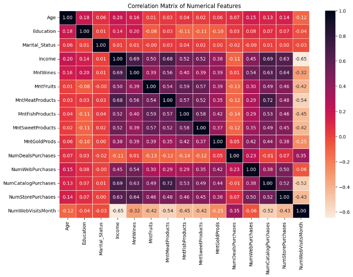
Exemple of insights :

NumDealsPurchases and Income (-0.11): This slightly negative correlation shows that higher-income customers tend to be less interested in purchasing via discounts, possibly indicating price insensitivity

Clustering

We employed K-Means clustering to segment the customer base. First, the Elbow Method was used to determine the optimal number of clusters:

Elbow Method for determining optimal clusters

The Elbow Method is a technique used to determine the optimal number of clusters (K) for K-Means clustering. The goal is to choose a K value that minimizes the sum of squared distances between each point and its assigned cluster center, known as the Sum of Squared Errors (SSE).

How it works :

1. Run K-Means for a range of values for K (e.g., from 1 to 10).
2. For each K, calculate the SSE.
3. Plot SSE against the number of clusters K. As K increases, SSE decreases because the points are closer to their centroids.
4. Look for an "elbow" in the plot: a point where the SSE starts decreasing at a slower rate. This point suggests the optimal number of clusters.

Mathematical formula :

We want to minimize the squared Euclidean distance between the data point x and its closest cluster centroid.

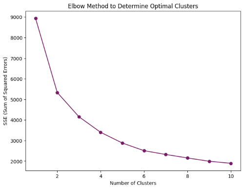
The Elbow Method suggested that 3 clusters would be optimal. After determining the number of clusters, K-Means was applied.

kmeans = KMeans(n_clusters=3, random_state=42)
df_cust['Cluster'] = kmeans.fit_predict(scaled_df)

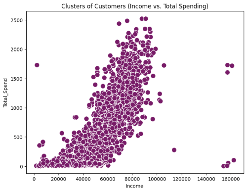
Here's the plot of unclustered points :

PCA and Clustering Comparison

To improve clustering performance and visualization, I applied Principal Component Analysis (PCA) to reduce the dataset’s dimensionality :

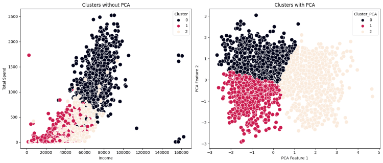
Comparison of Clustering with and without PCA:

Silhouette Score (be close to 1)

Without PCA: 0.31

With PCA: 0.40

Davies-Bouldin Index (be close to 0)

Without PCA: 1.19

With PCA: 0.88

Calinski-Harabasz Score (highest)

Without PCA: 1075.85

With PCA: 2133.39

Customer Segmentation

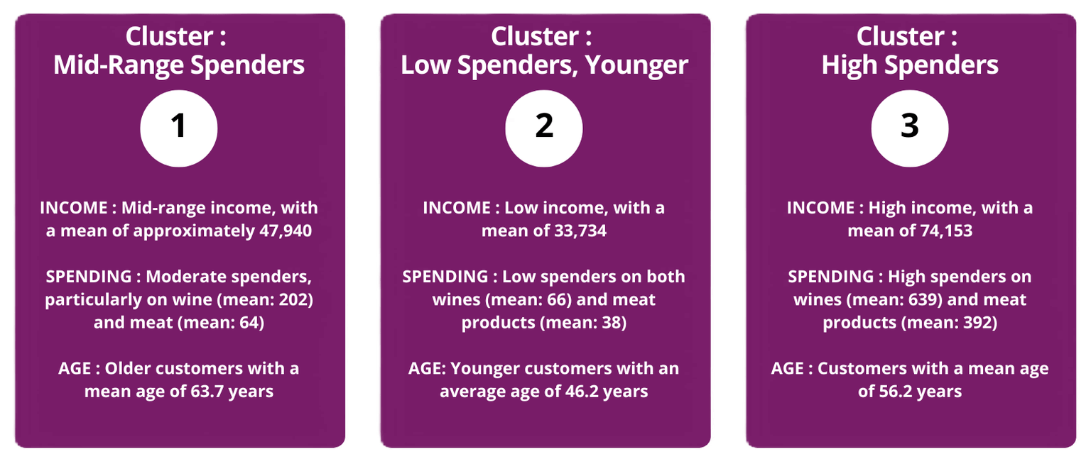
Based on the clusters formed, the customer segments were analyzed for their demographics and spending habits.

Marketing Recommendations

The final step is generating marketing recommendations based on the insights from each cluster:

• Cluster 0 (Mid-Range Spenders): Focus on value-based promotions such as bundled deals and loyalty programs.
• Cluster 1 (Low Spenders, Younger): Target these customers with price-sensitive promotions like discounts on frequently purchased items.
• Cluster 2 (High Spenders): Offer premium products and personalized campaigns focused on luxury items and VIP experiences.

General Recommendation

Tailor marketing strategies to fit each segment's spending patterns and preferences, such as offering premium products to high spenders or discounts to more price-sensitive customers.

Conclusion

This project showcased the power of customer segmentation through clustering. By understanding each customer segment’s income, spending patterns, and demographics, businesses can create more effective marketing strategies and enhance customer satisfaction.